Back in January, we presented our experimental feature for estimating aerobic threshold using HRV. Since this first implementation, we have worked considerably on the implementation of the method and can thus put to rest the original skepticism about how useful the determined values actually are.
The basic principle: Using the exact RR intervals between the individual heartbeats, the so-called DFA-alpha1 values are determined using non-linear mathematical methods. DFA stands for “Detrended fluctuation analysis” and alpha1 is the short term scaling exponent. It is known that this value changes with increasing intensity. From initial values above 1.0, the value decreases to about 0.75 at the aerobic threshold (not to be confused with the anaerobic threshold or lactate threshold!) and values around 0.5 at high intensity.
Notes
Before we go a little bit into the technical background of our implementation, we would like to get rid of some comments:
- The analysis of HRV data is very sensitive concerning single outliers. We would like to urge you to pay attention to the quality of the input data. Bruce Rogers has some recommendations in this regard in his FAQ listing. (Bluetooth should be used instead of ANT+; If there are 3% artifacts or more, the results are not trustworthy).
- Estimating Aerobic Threshold (or even Anaerobic Threshold, see DFA a1 and the HRVT2) should only be considered for dedicated ramp tests. Regression lines, as can be displayed in Runalyze, should only be considered when the activity solely involves a ramp test.
- The whole thing is a quite new topic. Despite our known time constraints, we will try to respond promptly as new information becomes available. Please remember: from our perspective, we are offering the feature as a beta feature to support current research.
- For the reason just mentioned, we are still far from catching up with the calculations for all existing activities. Therefore, we cannot show you long-term trends yet.
Technical implementation
There are three important steps for the determination of the DFA-alpha1 values:
- Detrending of RR intervals: Since the heart rate changes significantly over the course of an activity, the RR intervals are also subject to this long-term trend. This trend must be removed during preprocessing of the data. The method for this (see Tarvainen et al. 2002) is very simple in the mathematical formulation – very complex in the actual calculation.
- Artifact correction: As with all measurements, measurement errors can also occur during the acquisition of HRV data. These must first be detected and corrected or removed for further calculations. Here, there are potentially numerous methods of varying complexity and quality.
- Segment-wise calculation of DFA-alpha1 values: DFA is a “standard tool” of mathematics. Differences between different implementations should be minimal.
Runalyze is primarily written in PHP as a web application and accordingly we did the first implementation of the feature in January in PHP as well. Let me just tell you: More complex mathematical methods in PHP are a horror. What works in e.g. Python, R or MATLAB with only a few lines of code and little computing time, is complex and computationally intensive in PHP. Our first implementation therefore did without detrending (1) and used a simple method for artifact correction (2). The results were accordingly insufficient.
Our solution for detrending
In early May, we decided to invest the time and implement the method in R. With the RHRV package, a library is available here that already provides everything for (2) and (3), and detrending (1) is implemented in a few lines of code, as mentioned. The result was usable: The results were much closer to those of the Kubios software, which is considered the gold standard for HRV evaluations, so to speak.
The only problem: performance. Detrending requires finding the inverse of an NxN matrix, where N is the number of RR intervals. For 1h of activity at an average of 150bpm, that’s N = 9,000 values, which corresponds to a matrix with 81 million entries. Calculating the inverse is equivalent to solving a linear system of equations with 9,000 equations. What sounds complicated, computers can do pretty fast nowadays. But for a 3h activity we are already talking about 9 times the effort – and for a web application like Runalyze, response times of > 1s are already very annoying, not to mention the > 30s needed here at the beginning.
The solution: We also determine the detrending segment by segment (with some overlap). Our tests have shown that the bias (i.e. the systematic error we commit with this) is of negligible magnitude. Another advantage is that the NxN matrix and its inverse are initially independent of the RR intervals themselves, so we only need to compute the inverse once for numerous segments of length N. This means that we do not need to compute the inverse of the NxN matrix. In addition, we have implemented some methods of the RHRV package itself to achieve even better performance.
Our previous solution for artifact correction
Now, when we thought we were almost there, Bruce comparison between Runalyze and Kubios (and HRV logger) made us realize that our artifact correction (2) is insufficient. The RHRV package offers the FilterNIHR method, which uses time-dependent thresholds in a relatively similar way to the method used by Kubios (see Lipponen & Tarvainen 2019). Unfortunately, this internally restricts the thresholds to a fixed range, which may be useful for HRV data at rest, but is insufficient for activity data.
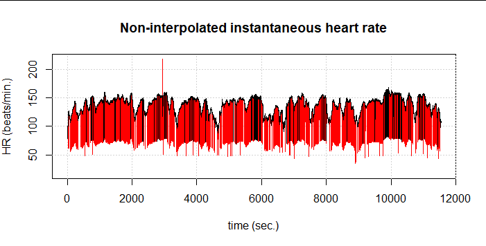
Here we see an example of a 3h cycling session without filtering (red) and with the RHRV filtering (black). The first thing to note is that the percentage of artifacts is incredibly high, although in the plot this is also due to the length of the activity: out of 25,003 data points, FilterNIHR detects 1,350 artifacts (5.4%). We see in black, however, that other obvious artifacts were not detected.
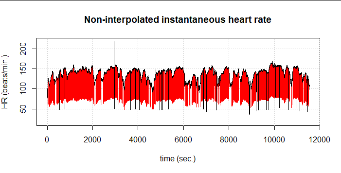
Therefore, we had to partially give away our elaborately gained performance and again choose the more computationally intensive implementation as presented by Kubios and Lipponen & Tarvainen. The result is 1,485 detected artifacts (5.9%). Still, some artifacts remain undetected:
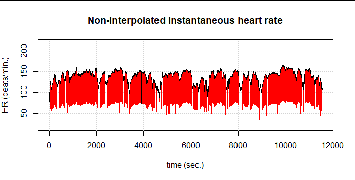
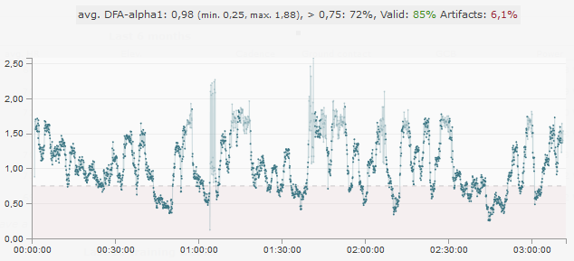
If we now combine both methods, i.e. first the one from Lipponen & Tarvainen and then again FilterNIHR, 1,516 artifacts (6.1%) are detected. At first glance, only one undetected artifact remains:
So even this combined method does not quite manage to really capture all artifacts correctly. We also see the effect in the resulting DFA-alpha1 values (at 120s window width and 115s overlap). At about 1:05:00 comes an area where DFA-alpha1 jumps wildly between values at about 1 and about 2. In the graph, these values are slightly transparent because the segments in this case exceed the set limit of 10ms due to the high SDNN of about 43ms.
We are working on further refining the method to detect this artifact as well. Until then you should – as always – pay attention to the best possible input data. The fewer artifacts there are in the data, the lower the probability that individual artifacts will not be detected. In this example, we would not trust the results anyway because of the total percentage of artifacts of 6.1%.
Literature
- Gronwald, T., Rogers, B., Hoos, O.: Fractal Correlation Properties of Heart Rate Variability: A New Biomarker for Intensity Distribution in Endurance Exercise and Training Prescription?, Frontiers in Physiology, 11, p. 1152, 2020. doi:10.3389/fphys.2020.550572
- Rogers, B., Giles, D., Draper, N., Hoos, O., Gronwald, T.: A new detection method defining the aerobic threshold for endurance exercise and training prescription based on fractal correlation properties of heart rate variability, Frontiers in Physiology, 2020. doi:10.3389/fphys.2020.596567
- Rogers, B.; Giles, D.; Draper, N.; Mourot, L.; Gronwald, T.: Influence of Artefact Correction and Recording Device Type on the Practical Application of a Non-Linear Heart Rate Variability Biomarker for Aerobic Threshold Determination. Sensors 2021, 21, 821. doi.org/10.3390/s21030821
- Rogers, B.; Giles, D.; Draper, N.; Mourot, L.; Gronwald, T.: Detection of the Anaerobic Threshold in Endurance Sports: Validation of a New Method Using Correlation Properties of Heart Rate Variability. J. Funct. Morphol. Kinesiol. 2021, 6, 38. doi.org/10.3390/jfmk6020038
There is also a wealth of information on the subject on Bruce Rogers’ blog.